Overfitting

Overfitting: Why Betting Models That Backtest Brilliantly Lose Real Money

Your spreadsheet says you'd have made a fortune last season. Here's why it's probably lying, and the honest tests that separate a real edge from a beautiful accident.

Overfitting: Why Betting Models That Backtest Brilliantly Lose Real Money
On this page

Overfitting: the backtest that lied

You've spent the summer building a football model. Form over the last five, home and away splits, shots, a dash of referee data, and a filter for odds between 3.20 and 3.60. You run the backtest over last season's Premier League and it spits out a +25% return. You're already browsing for a new car.

Then the season kicks off and the thing bleeds money from the first weekend.

It's the most familiar story in betting analytics, and it has a name: overfitting. The model didn't find an edge. It found last season. Every quirk, every fluke goal, every rain-soaked Tuesday win got baked in as though it were a law of football, and none of it comes round again.

Here's the good part. Overfitting is beatable, and the fixes are simple even if they're not glamorous. Keep the future out of your data. Count how many ideas you've tried. Test on matches the model has never seen, score probabilities properly and measure everything against the closing line. Do that and you'll know whether your model works before the bookies tell you the expensive way. Our line is blunt: if your model can't beat the closing line, it doesn't work.

The short version

A backtest that looks brilliant has usually found last season, not an edge. Keep the future out of your data, count every idea you try and test on matches the model has never seen. Then put your probabilities up against de-margined closing odds: beat those consistently and you might have something real.

Overfitting explained: memorising last year's exam paper

"Is the monkey who typed Hamlet actually a good writer?"
— Model Selection and Model Averaging (2008)

That line gets right to it. A model that fits the past perfectly hasn't necessarily learned a thing, any more than a monkey bashing out Shakespeare by chance is a playwright. Statisticians define overfitting as an analysis that corresponds "too closely or exactly to a particular set of data" and so fails to predict future observations reliably. In plain terms, the model has mistaken noise for structure.

Picture a student who memorises last year's exam paper word for word. Hand them the same paper and they score 100%. Hand them a new one and they're stuck. A betting model with dozens of features fitted to one Premier League season, just 380 matches and 38 per team, has far more freedom than that data can justify. It will cheerfully "learn" that Team X wins when it rains on a Tuesday.

Football makes it worse than most sports. Goals are rare, so single results are noisy, and over a few hundred bets a decent model and a lucky guess look almost identical. Push it to the extreme and a model with as many parameters as matches can reproduce the training data perfectly, then fall flat on the very next game.

The warning signs

  • The backtest is spectacular, the live results are ordinary. Some drop-off is normal (statisticians call it shrinkage), but a cliff edge isn't.
  • Nudge a threshold and the profit vanishes. Real edges survive small changes. Overfitted ones don't.
  • The winning rule is oddly specific. "Away teams, Mondays, odds 3.20 to 3.60" is the fingerprint of noise, not insight.

Underfitting is the opposite failure: a model too simple to catch real patterns, like drawing a straight line through a curve. The sweet spot is what Burnham and Anderson called the principle of parsimony, as simple as possible and only as complex as the data genuinely supports. For bettors we'd go further. Simple beats clever until clever proves itself out of sample.

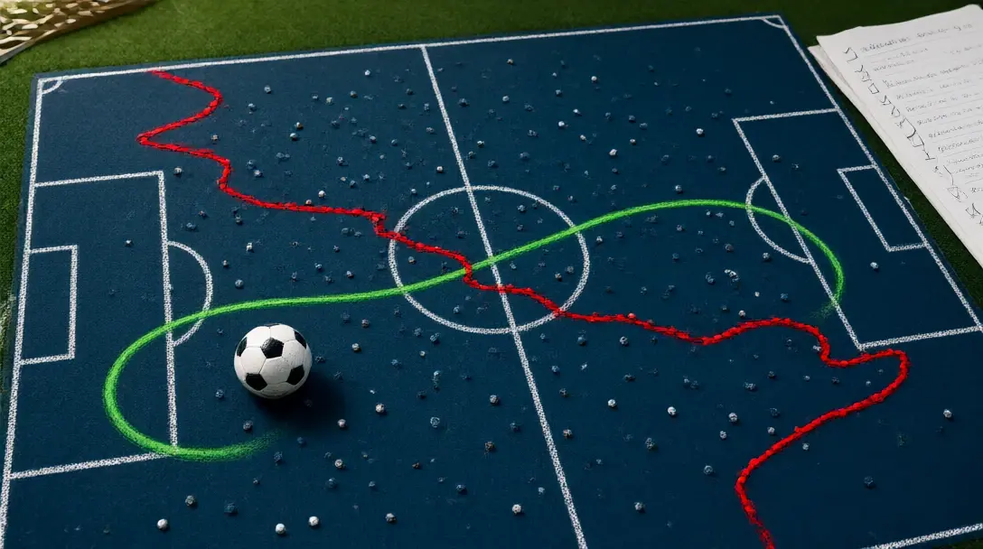
Scatter of dots over a football pitch with a jagged red line hitting every point and a smooth green curve through the middle
A line that hits every dot is memorising the past, not predicting the future.

Data leakage: the closing-odds trap

Leakage is overfitting's sneakier cousin. Your model gets fed information it could never have had at the moment you'd actually place the bet, and the backtest looks brilliant because it has effectively been reading tomorrow's paper.

The classic betting leak sits in the free historical data most hobbyists start with. Football-Data.co.uk's results files carry pre-match odds from a range of bookmakers and, using the same code with an extra "C", the closing odds too: B365CH is Bet365's closing home-win price, and the Pinnacle columns follow the same pattern (PSH for the pre-closing price, PSCH for the close). Closing prices are superb information. Use them as a feature and then "bet" at an earlier price, or claim value against a number you couldn't have taken, and your backtest is fiction.

So ask one question of every feature: at the exact moment I place this bet, could I have known this number?

Feature Known at bet time? Why it leaks
Closing odds, if you bet earlier No The market hasn't closed yet
xG, shots or possession for this match No They're produced by the game you're predicting
"Last five games" average including this match No The window has swallowed the result
End-of-season table or ratings No Built partly from future matches
Confirmed starting XI, betting days ahead No Teams are named about an hour before kick-off
Last five completed matches, odds when you bet Yes Genuinely available at the time

Two quieter leaks catch experienced modellers as well. Scaling or selecting features on the whole dataset before you split it lets future matches shape how past ones are read. And team-strength ratings estimated from the full dataset carry knowledge of results that hadn't happened yet. The fix is boring but bulletproof: time-stamp every feature and bin anything that arrives after your bet would have gone on.

Look-ahead bias: prices you could never have taken

Look-ahead bias is leakage's close relative, and it often hides in the odds column rather than the features. Backtest with prices updated after the team news, or with a fixture list restated after the fact, and you're quietly cheating.

The worst offender is the "best odds" column. Backtesting at the best price across twenty-odd bookmakers assumes you held accounts with all of them and that every one took your full stake. Life doesn't work like that. Kaunitz, Zhong and Kreiner's 2017 paper, Beating the bookies with their own numbers, reported a strategy that was profitable in a 10-year simulation on closing odds, a 6-month simulation on minute-by-minute odds and 5 months of real-money staking. They also described bookmakers limiting their accounts once they started winning.

There's the whole lesson. Even a strategy that works can run into prices and stakes you simply can't get. Backtest at a price you could realistically have taken, with the stake you'd realistically have been allowed, and treat anything above that as a bonus. If your model leans on machine learning, our guide to whether machine learning can beat the bookmakers is the natural next read.

“If you torture the data enough, nature will always confess.”

— Ronald Coase, Nobel Prize-winning economist

Data snooping: try 100 systems and one will look great

This is the trap almost everyone falls into, because you don't have to do anything wrong to land in it. You just have to try a lot of ideas.

Statisticians call it data dredging, data snooping or p-hacking. At the usual 5% significance level, one in twenty useless ideas will look "significant" by pure chance. Test enough of them and it's virtually certain some will. The maths is short:

Chance at least one of m useless tests looks significant
  = 1 - (1 - 0.05)^m

m = 20   ->  1 - 0.95^20  = 0.64   (64%)
m = 100  ->  1 - 0.95^100 = 0.994  (99.4%)

A simple simulation shows what that does to a betting system. Take one hundred systems that are pure noise, each placing 300 bets at decimal odds of 2.00 (evens in fractional terms), where the true chance of winning is 47.6% (a fair 50% with a typical bookmaker margin taken off). Every one of them has a built-in loss of about 4.8% per bet. Repeat the whole experiment 200 times and the best-looking system of the hundred shows a median return of about +9.3%.

True ROI per system         = 2.00 x 0.476 - 1  = -4.8%
SD of ROI over 300 bets     = 1.0 / sqrt(300)   ≈ 5.8 points
Best of 100 (median)        ≈ +9.3%
Distance from true value    ≈ 14.1 / 5.8        ≈ 2.4 standard deviations

That "winner" is luck and nothing else. And you don't need to build 100 systems on purpose to get there. Every time you swap leagues, tweak an odds band, change a form window or bolt on a feature and re-run, you've tried another system. You are your own multiple-testing machine.

How to defend yourself

Write down your hypothesis and your success metric before you look at the data. Keep a running count of every variant you try, and raise the bar as that count climbs; that's the thinking behind corrections like Bonferroni (divide your significance level by the number of tests) and the gentler Holm-Bonferroni. Favour models with few parameters and a footballing reason to exist. A shiny backtest can't manufacture an edge that isn't there, any more than staking systems like the Martingale can turn a losing bet into a winning one.

Wall of small grey monitors with a single screen glowing green, a silhouetted analyst and a pair of dice in front
Try a hundred systems and one will look brilliant by luck alone.

Walk-forward validation: split by time, guard the final season

Never shuffle matches randomly into training and test sets. A random split lets the model learn from games played after the ones it's being tested on, which is a leak in its own right, and it mixes the same teams' form into both piles. In betting, time is the only honest way to cut the data.

The standard method is walk-forward validation. Train on seasons one to five, test on season six. Then train on one to six, test on seven, and keep rolling. Tune your settings on those validation seasons and nowhere else. Each step mirrors exactly what you'll face for real: everything known up to today, then a run of matches you've never seen.

Then comes the final exam. Hold back the most recent season and leave it alone while you build. You get one look. Peek, tweak and look again, and it isn't unseen any more. It has turned into another validation set, and you're overfitting through your own decisions, one innocent tweak at a time.

After that comes the gold standard: paper trading. Record your forecasts before kick-off, time-stamped, for a few hundred matches before a penny goes on. Seven weeks into the 2026/27 season, the current campaign is nowhere near big enough to judge a model on its own, and that's exactly the point. You need hundreds of genuine out-of-sample forecasts, not a hot start. Our complete guide to building a betting model walks through setting up that pipeline from scratch.

Brier score and log loss: accuracy is the wrong score

Ask most people how good their model is and they'll quote accuracy: how often the top pick won. For betting, that's close to useless. Back the favourite every week and you'll look very "accurate", but the odds already price the favourite in, so you earn nothing. What pays is getting the probability right, especially where yours differs from the market's.

That's calibration. When you say 40%, does it happen about 40% of the time? Three scores measure it properly, and all of them are "proper" scoring rules, meaning your expected score is best when you report what you genuinely believe.

Brier score (one yes/no event)  = (p - o)^2
  70% forecast, it happens:       (0.7 - 1)^2 = 0.09
  70% forecast, it doesn't:       (0.7 - 0)^2 = 0.49
  Always saying 50%:              0.25  (the "know-nothing" mark)

Log loss = -ln(probability you gave to what actually happened)
  80% on the winner:  0.22      8% on the winner:  2.53

RPS (three-way, ordered Home / Draw / Away)
  = 1/2 x [ (pH - oH)^2 + (pH + pD - oH - oD)^2 ]

Brier, introduced by Glenn Brier in 1950, is the mean squared error of your probabilities, and lower is better. Log loss is brutal on confident misses. The Rank Probability Score respects the fact that a home win is "closer" to a draw than to an away win, and Constantinou and Fenton argued in 2012 that it's the rule that properly assesses football forecasting models.

Take an illustrative match with three forecasters: a sensible model (55/25/20), the market (45/28/27) and an overconfident model (80/12/8).

Result Model RPS Market RPS Overconfident RPS Overconfident log loss
Home win 0.121 0.188 0.023 0.22
Draw 0.171 0.138 0.323 2.12
Away win 0.471 0.368 0.743 2.53

Illustrative numbers. Lower is better.

The overconfident forecaster looks a genius when the home side wins and gets hammered otherwise. Accuracy would score the 55% and 80% forecasts identically. Only averages over hundreds of matches reveal who's calibrated, so pair the scores with a calibration table: bucket your forecasts (0-10%, 10-20% and so on) and check the hit rate in each.

Why it matters for profit

Walsh and Joshi put this to the test on NBA data, training models over several seasons and running betting experiments on one held-out season with published odds. Choosing models by calibration returned an average +34.69%, against -35.17% when choosing by accuracy. It's basketball and a single test season, so take it as strong backing for the principle rather than a recipe. But it's a principle we'd build every model around: score probabilities, not picks.

The only benchmark that matters: the closing line

Every scoring rule needs a rival, and the toughest one going is free: the bookmaker's closing price with the margin stripped out. Turn the odds into probabilities first, then remove the overround.

Illustrative prices: Home 2.20, Draw 3.40, Away 3.50

Implied:  1/2.20 = 45.45%   1/3.40 = 29.41%   1/3.50 = 28.57%
Total  =  103.44%  -> overround 3.44%

Fair:     45.45 / 103.44 = 43.94%
          29.41 / 103.44 = 28.43%
          28.57 / 103.44 = 27.62%

Run your Brier, log loss and RPS on those fair closing probabilities over the same matches as your model. If your model doesn't beat them, it adds nothing the market doesn't already know, and you're paying the margin for the privilege. The close is so hard to beat because it has soaked up the team news and the sharpest money. Pinnacle itself says its limits rise from around $3,000 on early NFL lines to over $100,000 by kick-off as the numbers firm up.

That doesn't make the close unbeatable. Kaunitz and colleagues claimed to beat it in simulation, and Hubacek, Sourek and Zelezny's 2019 study argued that a model has to deliberately decorrelate from the bookmaker, because one that merely echoes the odds can't find value. Beating the close consistently is rare, and that's exactly why it's the right bar.

Track closing line value (CLV) on every bet

Closing line value compares the price you took with the final one. Pinnacle calls consistently beating the close "one of the strongest indicators" of a sharp bettor, and it reads far faster than profit, which is too noisy to trust early. A rough rule for odds near 2.00 shows why:

CLV = odds taken / closing odds
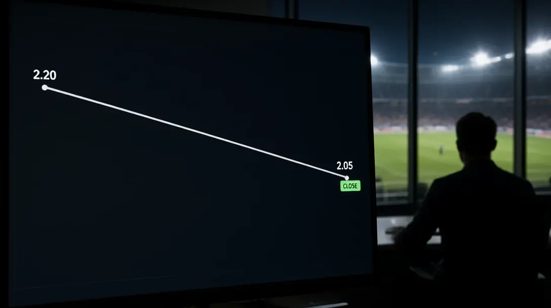
You take 2.20, it closes 2.05:  2.20 / 2.05 = 1.073  -> +7.3%

Bets needed to tell an edge from luck (about 95% confidence)
  ≈ (2 x SD per bet / edge)^2
  SD per bet at odds 2.00 ≈ 1.0
  5% edge:  (2 x 1.0 / 0.05)^2 = 40^2 = 1,600 bets

That's around 1,600 bets to prove a 5% edge on results alone, more than most punters will ever log. Positive CLV across a few hundred bets tells you far sooner whether you're on to something, which is why it sits at the heart of proper value betting.

Odds screen showing a price falling from 2.20 to 2.05 with a CLOSE marker, a floodlit stadium behind a silhouetted trader
Take 2.20, watch it close at 2.05: that gap is closing line value.

Our angles for building a betting model that lasts

  • Beat the close or bin it. If your fair probabilities don't out-score de-margined closing odds, your model is a hobby, not an edge.
  • Time-stamp everything. Any feature you couldn't have known when the bet went on is a leak, and leaks turn every backtest into a hero.
  • Count your attempts. Twenty tweaks means a 64% chance something looks great by accident. Raise the bar as the count climbs.
  • Split by time, never at random. Walk forward season by season and give the most recent season exactly one look.
  • Score probabilities, not picks. Brier, log loss and RPS plus a calibration table will tell you more than any strike rate.
  • Backtest at prices you could really get. Best-odds-across-the-market backtests ignore limits and restricted stakes.
  • Paper-trade first, then stake small. A few hundred time-stamped forecasts with positive CLV are worth more than any backtest you'll ever run.

Whatever your model says, keep stakes to a fixed, affordable slice of your bank and never chase a bad week by raising them.

Topics